How big is a Hilbert Space?

by Anastasiya Khromova, Dr.rer.nat, (originally published on Medium Jun 5, 2023, https://medium.com/@anastasiya.khromova17/how-big-is-a-hilbert-space-b925305b4d9b)

When a question has no correct answer, there is only one honest response.The gray area between yes and no. Silence.
Dan Brown, The Da Vinci Code

Yes (True) and No (False), Boolean. Or knowing as much as can be known as an alternative (the grey area, Quantum Mechanics).

In Hilbert space, nobody can hear you scream (Silence).
Ref. [1], [2].

Hilbert space is a special kind of vector space, it has all the properties of a regular vector space, like vector addition and scalar multiplication operation, but Hilbert space also has an inner product operation.

Vector space is a set of vectors ∣ψ₁⟩, ∣ψ₂⟩, ∣ψ₃⟩ … and associated scalars a₁, a₂, a₃… and consists of the operations of vector addition and scalar multiplication.

In math, a space is a set (a “universe”) with some added structure. The set comprises different mathematical objects such as vectors, numbers, points in space, variables, other sets, etc. The structure, a mathematical structure, or mathematical logic, is how the objects interact with each other, the relation/transformation, that acts on one or more sets to produce another set. It is the relation/transformation that defines the nature of the space.

Mathematical Space

Three notions are fundamental to the field of functional analysis, namely metric spaces, normed linear spaces, and inner product spaces. A metric space is simply a collection of objects (e.g. numbers, matrices, etc.) with an associated rule, or function, that determines the “distance” between two objects in the space. Such a function is termed a metric [3].

Definition (Metric Space). A metric space (X, d) is a set X together with an assigned metric function d: X × X → ℝ that has the following properties:

Positive: d(x, y) ≥ 0 for all x, y, z ∈ X
Non-degenerate: d(x, y) = 0 if and only if x = y
Symmetric: d(x, y) = d(y, x) for all x, y, z ∈ X
Triangle Inequality: d(x, z) ≤ d(x, y) + d(y, z) for all x, y, z ∈ X.

Perhaps the most intuitive example of a metric space is the real number line with the associated metric |x − y|, for x, y ∈ ℝ, where ℝ is a set of real numbers.

Normed linear spaces and inner product spaces, are simply special cases of metric spaces.

Definition (Normed Linear Space). A (complex) normed linear space (L,∥·∥) is a linear (vector) space with a function ∥·∥ : L → ℝ called a norm that satisfies the properties:

Positive: ∥v∥ ≥ 0 for all v ∈ L,1

2. Non-degenerate: ∥v∥ = 0 if and only if v = 0

3. Multiplicative: ∥λv∥ = |λ| ∥v∥ for all v ∈ L and λ ∈ ℂ

4. Triangle Inequality: ∥v + w∥ ≤ ∥v∥ + ∥w∥ for all v, w ∈ L

Definition (Inner Product Space). If V is a linear space, then a function ⟨·,·⟩ : V × V → ℂ is said to be an inner product provided that

1. Positive: ⟨v, v⟩ ≥ 0, for all v ∈ V

2. Non-degenerate: ⟨v, v⟩ = 0 if and only if v = 0

3. Multiplicative: ⟨λu, v⟩ = λ ⟨u, v⟩, for all u, v ∈ V and λ ∈ ℂ

4. Symmetric: ⟨u, v⟩ = ⟨v, u⟩*, whenever u, v ∈ V, Hermitian symmetry

5. Distributive: ⟨u + w, v⟩ = ⟨u, v⟩ + ⟨w, v⟩, for all u, w, v ∈ V

inner product space ⇒ normed linear space ⇒ metric space

Can we reverse the direction of these implications? No, we cannot. Does normed linear space imply inner product space? The answer is a very definitive no.

The l^ᵖ spaces are a class of normed linear spaces that seem to hold a special place in functional analysis. For each p ∈ ℝ, where p > 1, l^ᵖ is the set of all sequences (xₙ) such that the series:

is convergent. The standard norm || · ||ₚ for l^ᵖ is given by

for each (xₙ ) ∈ lᵖ.

The l^² space is the only one of the notions of the spaces that happens to be an inner product space. This “space” of sequence played an important role in the naming of Hilbert Space.

The notion of the l^ᵖ space comes from none other than David Hilbert, and Hilbert was known to discuss the l^ᵖ spaces during some of his lectures. Owing to the l^ᵖ space’s uniqueness from its peers, Hilbert’s students often referred to it as Hilbert’s space, from which we have the term Hilbert space [4].

One property that is common to all l^ᵖ spaces is that they are all normed linear spaces. The proof of this claim relies on Minkowski’s Inequality. Minkowski’s inequality tells us that || · ||ₚ satisfies the triangle inequality (indeed, Minkowski’s inequality can be thought of as the triangle inequality for l^ᵖ). Another common property is that all l^ᵖ spaces are complete. See Ref. [3] for details.

Cauchy sequences and complete metric spaces are defined in the following manner:

Definition (Cauchy Sequences). Let (aₙ) be a sequence in a metric space (X, d). The sequence (aₙ) is said to be Cauchy if for every ε > 0, there exists N ∈ ℕ such that d(aₙ, aₘ) < ε whenever n, m > N.

Definition (Complete Metric Space). If every Cauchy sequence in a metric space X converges to an element of X, then X is said to be complete.

Theorem. All l^ᵖ spaces are complete.

Hilbert Space. Not all normed or inner product spaces are complete. For this reason, we want to be able to distinguish complete normed or inner product spaces from those that are not, which is the motivation behind the definition of Banach and Hilbert spaces.

Definition (Banach Space). A Banach space is a completely normed linear space.

Definition (Hilbert Space). A Hilbert space is a complete inner product space.

Not all Banach spaces are Hilbert spaces. Specifically, while all lᵖ spaces are Banach spaces, only l² is a Hilbert space. Is there an inner product space that is not a Hilbert space? Are all inner product spaces necessarily complete? The answer is NO. Consider the set ℚ of rational numbers. Normal multiplication on rational numbers is a function that maps from ℚ×ℚ to ℚ ⊂ ℝ and satisfies all four of the criterion of Definition on Inner Product Space. However, the sequence (sₙ) of rational numbers, whose n term is given by

that converges to an irrational number π²/6 (Leonhard Euler). Since (sₙ) is convergent, and therefore Cauchy, we can safely conclude that while ℚ is an inner product space, it is not a Hilbert space. And there are also examples of a normed linear space that are not complete.

Quantum logic is a set of rules for the manipulation of propositions inspired by the structure of quantum mechanics. The propositional calculus of quantum mechanics has the same structure as an abstract projective geometry. Projections on a Hilbert Space can be viewed as propositions about physical observables. Principles for manipulating these quantum propositions were then called quantum logic by von Neumann and Birkhoff in a 1936 paper [5].

Definition (Compatible Propositions).
Two propositions p and q in a logic L are called compatible if there exist u, v, w ∈ L such that if {u, v, w} is a pairwise orthogonal set in L, then u ∨ v = p and v ∨ w = q.

The set {u, v, w} is called a compatibility decomposition for p and q.

Definition (Quantum Logic).
A quantum logic is a logic with at least two propositions that are not compatible.

Definition (Classical Logic).
A classical logic is a logic in which every pair of propositions is a compatible pair.

Properties of Hilbert Spaces

Types of Hilbert Spaces

There are two types of Hilbert Spaces, finite-dimensional and infinite-dimensional.

— Examples of finite-dimensional Hilbert spaces include [https://mathworld.wolfram.com/HilbertSpace.html], for n basis vectors:

1. The real numbers ℝⁿ with ⟨u, v⟩ the vector dot product of u and v.

2. The complex numbers ℂⁿ with ⟨u, v⟩ the vector dot product of u, and the complex conjugate of v.

The inner product on ℝⁿ is a typical dot product. Let’s two vectors:

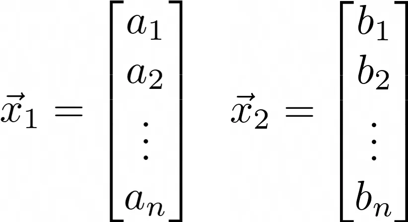
Then the vector dot product is:

Inner product on ℂⁿ, the complex inner product for two complex vectors:

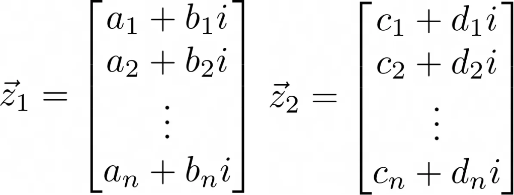
where i^²=-1. The inner product is then:

This formula extends for vectors of any length.

— An example of an infinite-dimensional Hilbert space is L² (a square-integrable function, or quadratically-integrable function), the set of all functions f: ℝ→ ℝ such that the integral of f² over the whole real line is finite. In this case, the inner product is:

An infinite-dimensional vector function is a function whose values lie in an infinite-dimensional topological vector space, such as the Hilbert Space or the Banach Space. There are two infinite-dimensional cases of the Hilbert Stace, corresponding to being separable (having a countable dense subset) or not.

Quantum Mechanical Logic

The classical and quantum worlds have some important things in common. Quantum mechanics, however, is different in two ways [7]:

Different Abstractions. Quantum abstractions are fundamentally different from classical ones. For example, we’ll see that the idea of a state in quantum mechanics is conceptually very different from its classical counterpart. States are represented by different mathematical objects and have different logical structures.
States and Measurements. In the classical world, the relationship between the state of a system and the result of a measurement of that system is very straightforward. In fact, it’s trivial. The labels that describe a state (the position and momentum of a particle, for example) are the same labels that characterize measurements of that state. In other words, you can measure them directly. In the quantum world, this is not true. States and measurements are two different things, and their relationship is subtle and non-intuitive.

The state of a quantum system.

According to the Copenhagen interpretation [8]:

A1. A pure state in quantum mechanics is represented in terms of a normalized vector |ψ⟩ in a Hilbert Space ℋ (a complex vector space with an inner product): ⟨ψ|ψ⟩ = 1. Suppose two states |ψ₁⟩ and |ψ₂⟩ are physical states of the system. Then their linear superposition c₁|ψ₁⟩ + c₂|ψ₂⟩ (cₖ ∈ ℂ) is also a possible state of the same system. This is called the superposition principle.

A state is a complete description of a physical system. In quantum mechanics, a state is a ray in a Hilbert Space. The phase of the vector may be chosen arbitrarily; |ψ⟩ represents the “ray” {e^iα |ψ⟩ |α ∈ ℝ}. In few words, we can totally ignore the overall phase of a vector since it has no observable consequence. For example, neither the probability |⟨λₖ |ψ⟩|² nor the average ⟨ψ|A|ψ⟩ depends on the phase and |ψ⟩ and e^iα|ψ⟩ describe the same state, where |e^iα | = 1. However, the relative phase of two different states IS meaningful. Although |⟨φ|e^iαψ⟩|² is independent of α, |⟨φ|ψ₁ + e^iα ψ₂⟩|² does depend on α.

A2. For any physical quantity (i.e., observable) a, such as energy, spin, position, and momentum, there exists a corresponding Hermitian operator A acting on the Hilbert Space ℋ. When we measure a in the state |ψ⟩, we obtain one of the eigenvalues λⱼ of the operator A and the state undergoes an abrupt change to the corresponding eigenvector |λⱼ⟩. This phenomenon is called the collapse of wave function. If we prepare an ensemble of many identical states |ψ⟩ and measure a, the probability of obtaining the outcome |λⱼ ⟩ is pⱼ = |⟨λⱼ|ψ⟩|². In quantum mechanics, an observable is a self-adjoint operator.

If in classical physics a physical variable, such as the energy or a component of angular momentum always has a well-defined value for a physical system in a particular state, in quantum physics this is no longer the case. If a quantum system is in the state |ψ⟩, the physical variable corresponding to the operator A has a well-defined value if and only if |ψ⟩ is an eigenvector of A:

where λⱼ is a scalar (usually complex) number. In these equations, the action of the operator A on the state vector |ψ⟩ returns the same state vector multiplied by the scalar λⱼ. This type of operator equation is known as an eigenvalue equation. Compared to the general operator equations of the form:

Operators play a particularly important part in quantum mechanics as will be shown below.

A (Boolean) bit assumes two distinct values, 0 and 1. Bits constitute the building blocks of the classical information theory (C. Shannon). A qubit is a (unit) vector in the vector space ℂ², whose basis vectors are denoted as:

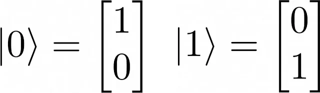
What these vectors physically mean depends on the physical realization employed for quantum-information processing: horizontally/vertically polarized photon, spin states of an electron, the ground state, and the first excited state of ionic energy levels or atomic energy levels.

In quantum mechanics the Dirac notation is used: the ket vector |ψ⟩ and the bra vector ⟨ψ| =[|ψ⟩*]^T (complex conjugate and transpose of |ψ⟩). The state of a single qubit is always a linear combination of the basis vectors |0⟩ and |1⟩

where where α and β are complex numbers and |α|²+|β|²=1.

Inner Product Properties in the Hilbert Space.

Braket ⟨ψ|ψ⟩ represents the inner product in the Hilbert Space and the properties of bras, let’s, and brakets are the following:

—Every |ψ⟩ has a ⟨ψ|

— |aψ⟩=a|ψ⟩, but ⟨aψ|=a*⟨ψ|

Conjugate symmetry: ⟨ψ|φ⟩ = ⟨φ|ψ⟩*
Linearity with respect to the second vector: ⟨ψ, a₁φ₁+a₂φ₂⟩ = a₁⟨ψ,φ₁⟩ +a₂⟨ψ, φ₂⟩
Anti-linearity with respect to the first vector: ⟨a₁ψ₁+a₂ψ₂, φ⟩ = a₁*⟨ψ₁, φ⟩ +a₂*⟨ψ₂, φ⟩
Norm is positive-definite: ⟨ψ|ψ⟩ = |ψ|² ≥ 0, =0 only if |ψ⟩=0

— Triangular inequality: √⟨ψ+φ| ψ+φ⟩ ≤ √⟨ψ|ψ⟩+√⟨φ|φ⟩

—Schwarz inequality: [⟨ψ|φ⟩]² ≤ [⟨ψ|ψ⟩] [⟨φ|φ⟩]

— Orthogonality and Orthonormality: ⟨ψ|φ⟩=0, ψ and φ are orthogonal, plus ⟨ψ|ψ⟩=1, ⟨φ|φ⟩=1 (unit vector of length 1)— vectors are orthonormal.

The inner product space has a dimension equal to the maximum number of nonzero, mutually orthogonal vectors it contains. Any collection of N mutually orthogonal vectors of length 1 in an N-dimensional vector space constitutes an orthonormal basis for that space. For many purposes, it is convenient to use normalized vectors but this is not always the case, or not any vector representing a quantum system must be normalized [9].

Operators and their Properties.

Operators are very useful tools also in classical mechanics. It is a function over a space of physical state onto another space of physical state (group theory, symmetry). Operator is a transformation (mapping) of one vector in the space onto another vector in that space. The function of an operator is to “generate” one state from another.

where the state vector |ϕ⟩ belongs to the same Hilbert space.

1. Linear operators are those operators that for any arbitrary pair of state vectors (of functions) |ψ₁⟩ and |ψ₂⟩ and scalar c obey the following properties:

The linearity of operators has several important consequences. Remember A1. above that, any state vector |ψ⟩ can be expressed as a linear combination of a complete set of basis states {|ϕᵢ⟩,i=1,2,3,…,n} associated to this Hilbert space:

where the values of the coefficients cᵢ can be fixed thanks to the orthogonality properties of the basis, ⟨ϕᵢ|ϕⱼ⟩=δᵢⱼ. Then one can see that for linear operators the following applies:

This result tells us that if we know the effects of the operator A for each of the elements of the basis |ϕᵢ⟩, we can easily determine its effect on a general state vector |ψ⟩ belonging to the same Hilbert space: the action of the operator A on the basis vectors {|ϕᵢ⟩} correlates with its action on any other state vector |ψ⟩ to which the operator was applied [10].

When we represent state vectors as operators in terms of components (matrix representation), we assume a choice of basis. If we change the basis, the values of the components will change too. The components of the operator in the matrix representation are defined as:

in the set of basis vectors {|ϕᵢ⟩,i=1,2,3,…,n}.

The values of e.g. A₁₁, A₁₂,… are basis-dependent.

But the eigenvector/operator relation depends only on the operator and vectors in question, and not on the particular basis in which they are expressed, basis-independent [9].

2. In general, operators are non-commutative, meaning that the order in which they are applied will vary the result of the operation.

3. Associative property:

4. Power property:

5. The long bracket (a scalar), with an operator sandwiched between a bra-vector and a ket-vector is a complex vector.

Operator acting on |ψ⟩ results in another vector |ψ⟩’, so at the end we obtain the inner product of two vectors which is another complex number.

6. The expectation value, or the mean value, of an operator with respect to the state |ψ⟩ is given by the following formula:

Operators could have the mean values because they represent the physical observables.

7. An interesting property is the outer product (a dyad) [11]:

In contrast to the inner product, which is a scalar, this mathematical construct is an operator (a linear operator). The dyads are i.e. the density operator |ψ⟩⟨ψ|, the projection operator, or the identity operator 𝕀, etc.

Types of Operators

There are many types of important operators in quantum mechanics.

Hermitian Operator Adjoint/Conjugate

For each vector state ket |Ψ⟩, there exists the corresponding bra vector ⟨Ψ| which can be understood as its complex conjugate. When expressing |Ψ⟩ as a column vector in terms of its components, ⟨Ψ| was the associated row vector expressing the complex conjugate of its components. In the case of operators, the story is different:

The correct relation is:

The operator with the dagger is known as the Hermitian adjoint of \hat{A}.

The action of the Hermitian adjoint operator on a ket vector?

The complex conjugate of the previous expression is:

Usually in QM, we are interested in operators that coincide with their Hermitian adjoints, meaning Hermitian operators.

2. The Hermitian operator is assigned to a physically observable property of a system, such as momentum, energy, angular momentum, position, etc. For example, the operator representing the energy is the Hamiltonian H.

Therefore, the Hermitian operator is an operator that is equal to its Hermitian conjugate:

A is anti-Hermitian if:

The terms “Hermitian” and “self-adjoint” mean the same thing for a finite-dimensional Hilbert space, which is all we are concerned with; the distinction is important for infinite-dimensional spaces [11].

3. The identity (or unit) 𝕀, zero (or null) operator and the Inverse operator. The zero (or null) operator is the operator that satisfies:

In the matrix representation the elements of zero operator are all zero.

The inverse and the identity operators have the following properties:

If you apply the sequence of the operator and its inverse the resulting operator is just and the identity operator. The inverse operators are useful when you divide two operators. The identity operator is a generalized version of the identity matrix where the diagonal elements are all unity while the off-diagonal elements vanish:

where δᵢⱼ is the Kronecker delta. This means that for a n-dimensional Hilbert space, the unit operator is the n-dimensional identity matrix. The unit operator has the same form in all representations irrespective of the specific choice of basis states. The identity operator can be given by the sum over the dyads |ϕᵢ⟩⟨ϕᵢ| corresponding to the elements |ϕᵢ⟩ of an orthonormal basis:

4. The unitary operator determines the time evolution of a quantum system. The operator is unitary if its Hermitian conjugate equals its inverse:

The product of two unitary operators is also unitary.

5. The projection operator can be defined as

where |Ψ⟩ is a normalized vector. The projection operator satisfies two conditions:

— it is Hermitian and

— it is equal to its own square which means that acting twice on a given state vector produces the same result as acting just once. This makes sense from a geometric viewpoint, since once you have projected a vector onto another vector, projecting the projection just gives you the same projection back again [9].

Applying the projection operator to any other vector |ϕ⟩ gives the projection of |ϕ⟩ along |Ψ⟩:

In analogy with the perpendicular projection in linear algebra, given two vectors |ϕ⟩ and |Ψ⟩, the perpendicular projection is the inner (dot) product of ⟨Ψ| with |ϕ⟩ and multiplying by the vector |Ψ⟩ when |Ψ⟩ is normalized (unit) vector.

Usually for projection operator, you use the letter P. They have the following properties:

If two projection operators P₁ and P₂ commute, meaning that their products are commutative,

then their product P₁P₂ and P₂P₁ is also a projection operator.

2. Two projection operators P₁ and P₂ are orthogonal projection operators if their product is zero: P₁P₂ = 0.

3. The sum of multiple projection operators typically is not a projection operator it still can be a projection operator as long as the projection operators within the sum are mutually orthogonal:

The operators in the sum are all orthogonal to each other.

The simplest type of measurement in quantum mechanics is the projective measurement, for a “perfect” measurement. The measurement operators of projective measurements are projectors, the projection operators. Remember the Axiom A2. Suppose Hilbert Space has dimension n, the ℂⁿ. The Hermitian operator A has a spectral decomposition [8]:

the λⱼ is an eigenvalue of the operator A and the scalar number. |ψ⟩ in terms of |λⱼ⟩ is

The probability of observing λⱼ upon measurement of an expectation value of a is |cⱼ|², and therefore the expectation value after many measurements is

Any particular outcome λⱼ will be found with the probability

|cⱼ|² = ⟨ψ|Pⱼ|ψ⟩,

where Pⱼ = |λⱼ⟩⟨λⱼ| is the projection operator, and the state immediately after the measurement is |λⱼ⟩ or equivalently

For example.

Let’s take the qubit system described by the state

and measure it in the |0⟩, |1⟩ basis. A measurement in the |0⟩, |1⟩ basis would then correspond to projectors onto each of the two states, M₀ = |0⟩⟨0| and M₁ = |1⟩⟨1|.

A measurement in quantum mechanics consists of a set of measurement operators

The probability of observing measurement outcome m is

2. The total probability over all measurement outcomes must sum to 1, therefore the completeness relation is:

where 𝕀 is the identity (unit) operator.

3. The state of the system immediately following the measurement is

The probability of measuring the system in state |0⟩ is:

And the state after measuring the system in |0⟩ is

Remember that the global phases don’t matter, the state after the measurement is simply |0⟩.

Conclusion for now

If our goal is to take a nature’s-eye view of things and specify the correct quantum theory of the world in its own right, to define that theory as a set of state vectors |Ψ⟩ in a Hilbert space H, evolving under the Schrödinger equation via a specified Hamiltonian Ĥ. The problem is that this is very little structure indeed. Hilbert space itself is featureless; a particular choice of Hilbert space is completely specified by its dimension d = dim H. A vector in Hilbert space contains no direct specification of what the physical content of such a state is supposed to be; there is no mention of space, configuration space, particles, fields, or any such familiar notions. Presumably all of that is going to have to somehow emerge from the dynamics, which seems like a tall order [1].

When working with ordinary 3-vectors (x, y, and z axes, Euclidean vector space), we have three mutually orthogonal unit vectors and use them as a basis to construct any vector. If you tried to find a 4th vector orthogonal to these three, there wouldn’t be any — not in 3-dimensions anyway. If there were more dimensions of space, there would be more basis vectors. The dimension of a space can be defined as the maximum number of mutually orthogonal vectors in that space [7]. The same principle is true for complex vector spaces.

A Hilbert space may have either a finite or an infinite number of dimensions. The simple spin is described by a two-dimensional space of states (qubit). For this reason, the observables have had only a finite number of possible observable values. However, there are more complicated observables that can have an infinite number of values. An example is a particle. The coordinates of a particle are observables, but, unlike spin, the coordinates have an infinite number of possible values. When the observables of a system are continuous, the wave function truly becomes a function of a continuous variable. To apply quantum mechanics to this kind of system, we have to expand the idea of vectors to include functions.

Functions are functions, and vectors are vectors — they seem like different things, so in what sense are functions vectors? If you think of vectors as arrows pointing in three-dimensional space, then they are not the same as functions. But if you take the broader view of vectors as a set of mathematical objects satisfying certain postulates, then functions can indeed form a vector space. Such a vector space is often called a Hilbert space [7].

[1] Reality as a Vector in Hilbert Space, Sean M. Carroll, https://doi.org/10.48550/arXiv.2103.09780

[2] Aharonov, Y., & Rohrlich, D. (2005). Quantum Paradoxes. Wiley, New York.

[3] A Brief Introduction to Hilbert Space and Quantum Logic, Joel Klipfel, https://www.whitman.edu/Documents/Academics/Mathematics/klipfel.pdf

[4] Saxe, Karen. Beginning Functional Analysis. New York: Springer. 2002.

[5] Birkhoff, Garrett and John von Neumann. The Logic of Quantum Mechanics. Annals of Mathematics 37, 823843. 1936.

[6] A very nice source, https://www.youtube.com/watch?v=7zx3MT9FgT0)

[7] Susskind, L. and Friedman, A., 2014, Quantum Mechanics: The Theoretical Minimum (2nd edition), New York: Basic Books.

[8] Quantum mechanics: Hilbert space formalism, Chi-Kwong Li, https://cklixx.people.wm.edu/teaching/QC2021/QC-chapter2.pdf

[9] Ismael, Jenann, “Quantum Mechanics”, The Stanford Encyclopedia of Philosophy (Fall 2021 Edition), Edward N. Zalta (ed.), https://plato.stanford.edu/entries/qm/#StruHilbSpac. Here you can also find a very nice suggestion for a Bibliography, for different levels of knowledge in Quantum Mechanics

[10] https://mathforquantum.quantumtinkerer.tudelft.nl/5_operators_QM/#51-definition-and-properties-of-operators

[11] Hilbert Space Quantum Mechanics, Robert B. Griffiths, https://quantum.phys.cmu.edu/QCQI/qmd111.pdf

M	T	W	T	F	S	S
1	2	3	4	5	6	7
8	9	10	11	12	13	14
15	16	17	18	19	20	21
22	23	24	25	26	27	28
29	30

Trieste Quantum Register

Experimental Quantum Optics, Quantum Technologies and Quantum Computer: theory, experiment, news

How big is a Hilbert Space?

Mathematical Space

Properties of Hilbert Spaces

Types of Hilbert Spaces